Join my course at Udemy (Python Programming Bible-From beginner to advanced )

Blogger templates

Showing posts with label Machine Learning. Show all posts

Wednesday, 13 May 2020

Principal Component Analysis (PCA) in R

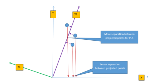
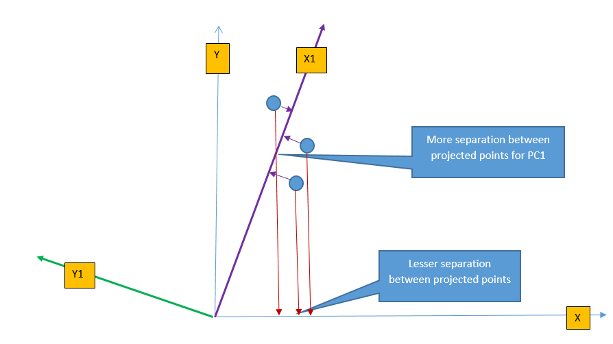
Principal Component Analysis (PCA) is unsupervised learning technique and it is used to reduce the dimension of the data with minimum loss of information. PCA is used in an application like face recognition and image compression. PCA transforms the feature from original space to a new feature space to increase the separation between data. The following figure shows the projection of three points on X-axis and X1-axis. It is easy to understand that projected points on X1-axis are better(more) separated than projected points on X-axis This is because the X1-axis is drawn in the direction of the highest variance of data points and so the projection of a point on this line results in maximum separation. PCA identifies the direction where the perpendicular distance from the data-point to the ‘maximum variance direction’ is smallest and projection of data on this line yields maximum separation.
Linear transformation, Dimension reduction & PCA

                             Z =∑{j=1}p ϕj * Xj
The above equation transforms the 'p' input feature X using co-efficient ϕ to Z. Please note that the transformed variable Z is a linear combination of ‘all’ input features X1, X2...Xp and none of the input features are discarded. The above equation can be extended to multiple dimension to create multiple transformed variable Z1, Z2, … Zm using a different set of a coefficient. Transformed variables Z1, Z2, … Zm will then be used for model building and if m<p then overall result will be a reduction in dimension from p to m.

Intuitively we can think of transformation as rotating the axis and taking the projection of data points. From the figure above, we can perform the linear transformation of data points by changing the axis from X to X1 and take the projection of data-points on X1-axis.

PCA changes the axis towards the direction of maximum variance and then takes projection on this new axis. The direction of maximum variance is represented by Principal Components (PC1). There are multiple principal components depending on the number of dimensions (features) in the dataset and they are orthogonal to each other. The maximum number of principal component is same as a number of dimension of data. For example, in the above figure, for two-dimension data, there will be max of two principal components (PC1 & PC2). The first principal component defines the most of the variance, followed by second principal component, third principal component and so on. Dimension reduction comes from the fact that it is possible to discard last few principal components as they will not capture much variance in the data. Following steps shows how to get the principal components:
  • Find the mean of each feature and then subtract observations from the mean for each of the features so that the origin is changed to the centroid. This is done to ensure that PC1 will pass through centroid origin, otherwise PC1 will still pass through centroid but this will not be the centroid. Please read through the reference [2] for more details.
  • Find the covariance matrix. This defines the correlation between different features in matrix form.
  • Then find the eigenvector and eigenvalue for the covariance matrix obtained in the previous step. Eigenvalues defines length of the eigenvector or the contribution of each principal component to defining the variance of the dataset.
It is possible that we will not take into account all principal component into consideration as PC1, PC2, ...PCp defines the order of variance and first, few principal components will be good enough to define the good proportion of variance. One thing to note that it may not be possible to get the meaning out of the new set of features as new features are linearly transformed features from the original set of features.

How to implement PCA in R

We will use the famous ‘iris’ data for PCA. This dataset has 4 numerical features and 1 categorical feature.
input = read.csv("iris.csv")
names(input)
str(input)
> names(input)
[1] "sepal_len" "sepal_wid" "petal_len" "petal_wid" "class" 
> str(input)
'data.frame': 150 obs. of  5 variables:
 $ sepal_len: num  5.1 4.9 4.7 4.6 5 5.4 4.6 5 4.4 4.9 ...
 $ sepal_wid: num  3.5 3 3.2 3.1 3.6 3.9 3.4 3.4 2.9 3.1 ...
 $ petal_len: num  1.4 1.4 1.3 1.5 1.4 1.7 1.4 1.5 1.4 1.5 ...
 $ petal_wid: num  0.2 0.2 0.2 0.2 0.2 0.4 0.3 0.2 0.2 0.1 ...
 $ class    : Factor w/ 3 levels "Iris-setosa",..: 1 1 1 1 1 1 1 1 1 1 ..

We will use prcomp function for PCA. The prcomp provides four output as dumped below.
  • Sdev – This defines the standard deviation of projected points on PC1, PC2, PC3 and PC3. As expected, the standard deviation of projected point is in decreasing order from PC1 to PC4.
  • Rotation – This defines the principal components axis. Here there are four principal components as there are four input features.
  • Center/Scale – These are mean and standard deviation of input features in original feature space (without any transformation).
model = prcomp(input[,1:4], scale=TRUE)
model$sdev
model$rotation
model$center
model$scale
model$sdev
[1] 1.7061120 0.9598025 0.3838662 0.1435538
> model$rotation
                 PC1         PC2        PC3        PC4
sepal_len  0.5223716 -0.37231836  0.7210168  0.2619956
sepal_wid -0.2633549 -0.92555649 -0.2420329 -0.1241348
petal_len  0.5812540 -0.02109478 -0.1408923 -0.8011543
petal_wid  0.5656110 -0.06541577 -0.6338014  0.5235463
> model$center
sepal_len sepal_wid petal_len petal_wid 
 5.843333  3.054000  3.758667  1.198667 
> model$scale
sepal_len sepal_wid petal_len petal_wid 
0.8280661 0.4335943 1.7644204 0.7631607
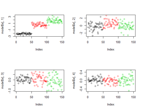
The following figure shows the plots of projected points on principal components. It is very clear that projected points on PC1 clearly classify the data but the plots of projected points by lower principal components (for PC2, PC3 & PC4) is not able to classify the data as convincingly as PC1.
par(mfrow=c(2,2))
plot(model$x[,1], col=input[,5])
plot(model$x[,2], col=input[,5])
plot(model$x[,3], col=input[,5])
plot(model$x[,4], col=input[,5])
           

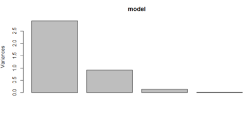
The following plots show the dominance of PC1. The bar graph shows the proportion of variance explained by principal components. We can see that PC1 explains 72% of the variance, PC2 explains 23% of the variance and so on. The same has been shown in the plot below. Please note that PC1 and PC2 together explain around 95% of the variance and we can discard the PC3 and PC4 because their contribution towards explaining the variance is just 5%.
model$sdev^2 / sum(model$sdev^2)
plot(model)
> model$sdev^2 / sum(model$sdev^2)
[1] 0.727704521 0.230305233 0.036838320 0.005151927


PCA without ‘prcomp’

The following code shows how to get the direction on principal components using eigenvector. Please note that eigenvector is same as the output of model$rotation using prcomp (in the previous example).
## Normalize the input feature. 
input$sepal_len1 = (input$sepal_len - mean(input$sepal_len) )/sd(input$sepal_len)
input$sepal_wid1 = (input$sepal_wid - mean(input$sepal_wid))/sd(input$sepal_wid)
input$petal_len1 = (input$petal_len - mean(input$petal_len))/sd(input$petal_len)
input$petal_wid1 = (input$petal_wid - mean(input$petal_wid))/sd(input$petal_wid)

##Get the covarience matrix and eigen vector.
matrix_form = matrix(c(input$sepal_len1, input$sepal_wid1, input$petal_len1, input$petal_wid1), ncol=4)
m = cov(matrix_form)
eigenV = eigen(m)
eigenV$vectors
       [,1]        [,2]       [,3]       [,4]
[1,]  0.5223716 -0.37231836  0.7210168  0.2619956
[2,] -0.2633549 -0.92555649 -0.2420329 -0.1241348
[3,]  0.5812540 -0.02109478 -0.1408923 -0.8011543
[4,]  0.5656110 -0.06541577 -0.6338014  0.5235463

Conclusion

PCA is very useful in reducing the dimension of data. Some important point to note before using PCA:
  • As PCA tries to find the linear combination of data and if the data in the dataset has non-linear relation then PCA will not work efficiently.
  • Data should be normalized before performing PCA. PCA is sensitive to scaling of data as higher variance data will drive the principal component.

Reference

Share:

Tuesday, 12 May 2020

Logistics Regression, LDA and QDA in R

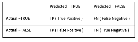
Classification algorithm defines set of rules to identify a category or group for an observation. There is various classification algorithm available like Logistic Regression, LDA, QDA, Random Forest, SVM etc. Here I am going to discuss Logistic regression, LDA, and QDA. The classification model is evaluated by confusion matrix. This matrix is represented by a table of Predicted True/False value with Actual True/False Value. The confusion matrix is shown as below. This list down the TRUE/FALSE for Predicted and Actual Value in a 2X2 table.

 From the above table, prediction result is correct for TP and TN and prediction fails for FN and FP. Following terms are defined for confusion matrix:
    True Positive Rate = TP / ( TP+FN ) – Defines proportion of TRUE (Actual=TRUE) observations that are predicted ( predicted as TRUE ) correctly. True Negative Rate = TN / ( TN+FP ) – Defines proportion of FALSE ( Actual=FALSE ) observations that are predicted ( predicted as FALSE ) correctly. Accuracy = TP+TN / (TP+TN+FP+FN) – Defines overall correct prediction result.

Classification Algorithm (Logistic regression, LDA & QDA)

Logistic Regression Logistic Regression is an extension of linear regression to predict qualitative response for an observation. It defines the probability of an observation belonging to a category or group. Logistics regression is generally used for binomial classification but it can be used for multiple classifications as well. Following is the equation for linear regression for simple and multiple regression.
    Y = β0 + β1 X + ε ( for simple regression ) Y = β0 + β1 X1 + β2 X2+ β3 X3 + …. + βp Xp + ε (for multiple regression )
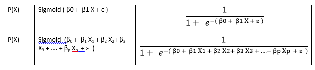
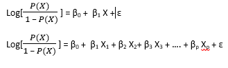
Linear Regression works for continuous data, so Y value will extend beyond [0,1] range. As the output of logistic regression is probability, response variable should be in the range [0,1]. To solve this restriction, the Sigmoid function is used over Linear regression to make the equation work as Logistic Regression as shown below.                                     The above probability function can be derived as function of LOG (Log Odds to be more specific) as below. From the equation it is evident that Log odd is linearly related to input X. The Log Odd equation helps in better intuition of what will happen for a unit change in input (X1, X2…, Xp) value. For example - a change in one unit of predictor X1, and keeping all other predictor constant, will cause the change in the Log Odds of probability by β1 (Associated co-efficient of X1)

Bayes Theorem, LDA (Linear Discriminant Analysis) & QDA (Quadratic Discriminant Analysis )

LDA and QDA algorithms are based on Bayes theorem and are different in their approach for classification from the Logistic Regression. In Logistic regression, it is possible to directly get the probability of an observation for a class (Y=k) for a particular observation (X=x). LDA and QDA algorithm is based on Bayes theorem and classification of an observation is done in following two steps.
    Identify the distribution for input X for each of the class (or groups ex Y=k1, k2, k3 etc ) Flip the distribution using Bayes theorem to calculate the probability Pr(Y=k|X=x)
                                                                     The above equation has following terms:
    Pr⁡(Y=k|X=x) - Probability that an observation belongs to response class Y=k, provided X=x. Pr(X=x|Y=k) - Probability of X=x, for a particular response class Y=k.
The distribution of X=x needs to be calculated from the historical data for every response class Y=k. In LDA algorithm, the distribution is assumed to be Gaussian and exact distribution is plotted by calculating the mean and variance from the historical data.
    Pr(Y=k) – a Prior probability that an observation is of particular class Y=k. ∑(Pr⁡(X=x|Y=p)*Pr⁡(Y=p)) – Sum of probability that an observation is of type X=x for all classes of Y.
In simple terms, if we need to identify a Disease (D1, D2,…, Dn) based on a set of symptoms (S1, S2,…, Sp) then from historical data, we need to identify the distribution of symptoms (S1, S2, .. Sp) for each of the disease ( D1, D2,…,Dn) and then using Bayes theorem it is possible to find the probability of the disease(say for D=D1) from the distribution of the symptom. LDA (Linear Discriminant Analysis) is used when a linear boundary is required between classifiers and QDA (Quadratic Discriminant Analysis) is used to find a non-linear boundary between classifiers. LDA and QDA work better when the response classes are separable and distribution of X=x for all class is normal. The more the classes are separable and the more the distribution is normal, the better will be the classification result for LDA and QDA. Following are the assumption required for LDA and QDA: LDA Assumption:
    Common covariance across all response classes σ2 ( for ex σk1 = σk2 = σk3 for k1, k2 , k3 response classes ) Distribution of observation in each of the response classes is normal with a class-specific mean (µk) and common covariance σ.
QDA Assumption:
    Different covariance for each of the response classes. For ex – σk1, σk2, σk3 for response class k1, k2, k3 etc. Distribution of observation in each of the response class is normal with a class-specific mean (µk) and class-specific covariance (σk2).

R Implementation

I will use the famous ‘Titanic Dataset’ available at Kaggle to compare the results for Logistic Regression, LDA and QDA.

Get the data and find the summary and dimension of the data

As a first step, we will check the summary and data-type. From the below summary we can summarize the following:
    Dataset has 891 rows and 12 columns. Out of the 12 columns, we can remove PassengerId, Name and Ticket based on the UniqueValue dump from the dataset. The dump shows that the three features are mostly unique for passengers. There is huge number of NA value for ‘Age’ (Almost 19.8 %, 177 out of 891) and so we can’t remove these rows. We will have a mechanism to replace the missing value for ‘Age’. ‘Cabin’ has huge number of missing value (687 out of 891) and so it will be better to not use this feature.
library(MASS)
library(ggplot2)
titanicDS = read.csv("train.csv")
dim(titanicDS)
[1] 891  12
str(titanicDS)
'data.frame': 891 obs. of  12 variables:
 $ PassengerId: int  1 2 3 4 5 6 7 8 9 10 ...
 $ Survived   : int  0 1 1 1 0 0 0 0 1 1 ...
 $ Pclass     : int  3 1 3 1 3 3 1 3 3 2 ...
 $ Name       : Factor w/ 891 levels "Abbing, Mr. Anthony",..: 109 191 358 277 16 559 520 629 417 581 ...
 $ Sex        : Factor w/ 2 levels "female","male": 2 1 1 1 2 2 2 2 1 1 ...
 $ Age        : num  22 38 26 35 35 NA 54 2 27 14 ...
 $ SibSp      : int  1 1 0 1 0 0 0 3 0 1 ...
 $ Parch      : int  0 0 0 0 0 0 0 1 2 0 ...
 $ Ticket     : Factor w/ 681 levels "110152","110413",..: 524 597 670 50 473 276 86 396 345 133 ...
 $ Fare       : num  7.25 71.28 7.92 53.1 8.05 ...
 $ Cabin      : Factor w/ 148 levels "","A10","A14",..: 1 83 1 57 1 1 131 1 1 1 ...
 $ Embarked   : Factor w/ 4 levels "","C","Q","S": 4 2 4 4 4 3 4 4 4 2 ...
summary(titanicDS)
  PassengerId       Survived          Pclass                                         Name    
 Min.   :  1.0   Min.   :0.0000   Min.   :1.000   Abbing, Mr. Anthony                  :  1  
 1st Qu.:223.5   1st Qu.:0.0000   1st Qu.:2.000   Abbott, Mr. Rossmore Edward          :  1  
 Median :446.0   Median :0.0000   Median :3.000   Abbott, Mrs. Stanton (Rosa Hunt)     :  1  
 Mean   :446.0   Mean   :0.3838   Mean   :2.309   Abelson, Mr. Samuel                  :  1  
 3rd Qu.:668.5   3rd Qu.:1.0000   3rd Qu.:3.000   Abelson, Mrs. Samuel (Hannah Wizosky):  1  
 Max.   :891.0   Max.   :1.0000   Max.   :3.000   Adahl, Mr. Mauritz Nils Martin       :  1  
                                                  (Other)                              :885  
     Sex           Age            SibSp           Parch             Ticket         Fare       
 female:314   Min.   : 0.42   Min.   :0.000   Min.   :0.0000   1601    :  7   Min.   :  0.00  
 male  :577   1st Qu.:20.12   1st Qu.:0.000   1st Qu.:0.0000   347082  :  7   1st Qu.:  7.91  
              Median :28.00   Median :0.000   Median :0.0000   CA. 2343:  7   Median : 14.45  
              Mean   :29.70   Mean   :0.523   Mean   :0.3816   3101295 :  6   Mean   : 32.20  
              3rd Qu.:38.00   3rd Qu.:1.000   3rd Qu.:0.0000   347088  :  6   3rd Qu.: 31.00  
              Max.   :80.00   Max.   :8.000   Max.   :6.0000   CA 2144 :  6   Max.   :512.33  
              NA's   :177                                      (Other) :852                   
         Cabin     Embarked
            :687    :  2   
 B96 B98    :  4   C:168   
 C23 C25 C27:  4   Q: 77   
 G6         :  4   S:644   
 C22 C26    :  3           
 D          :  3           
 (Other)    :186 
attach(titanicDS)
UniqueValue = function (x) {length(unique(x)) }
apply(titanicDS, 2, UniqueValue)
PassengerId    Survived      Pclass        Name         Sex         Age       SibSp 
        891           2           3         891           2          89           7 
      Parch      Ticket        Fare       Cabin    Embarked 
          7         681         248         148           4 
NaValue = function (x) {sum(is.na(x)) }
apply(titanicDS, 2, NaValue)
PassengerId    Survived      Pclass        Name         Sex         Age       SibSp 
          0           0           0           0           0         177           0 
      Parch      Ticket        Fare       Cabin    Embarked 
          0           0           0           0           0 
BlankValue = function (x) {sum(x=="") }
apply(titanicDS, 2, BlankValue)
PassengerId    Survived      Pclass        Name         Sex         Age       SibSp 
          0           0           0           0           0          NA           0 
      Parch      Ticket        Fare       Cabin    Embarked 
          0           0           0         687           2 
MissPercentage = function (x) {100 * sum (is.na(x)) / length (x) }
apply(titanicDS, 2, MissPercentage)
PassengerId    Survived      Pclass        Name         Sex         Age       SibSp 
    0.00000     0.00000     0.00000     0.00000     0.00000    19.86532     0.00000 
      Parch      Ticket        Fare       Cabin    Embarked 
    0.00000     0.00000     0.00000     0.00000     0.00000 

Process the missing value for ‘Age’.

The next step will be to process the ‘Age’ for the missing value. There are various ways to do this for example- delete the observation, update with mean, median etc. In the current dataset, I have updated the missing values in ‘Age’ with mean. Following code updates the ‘Age’ with the mean and so we can see that there is no missing value in the dataset.

titanicDS$Age[is.na(titanicDS$Age)] = mean(titanicDS$Age, na.rm=TRUE)
apply(titanicDS, 2, MissPercentage)
PassengerId    Survived      Pclass        Name         Sex         Age       SibSp 
          0           0           0           0           0           0           0 
      Parch      Ticket        Fare       Cabin    Embarked 
          0           0           0           0           0 
Now our data is data is ready to create the model. As a first step, we will split the data into testing and training observation. The data is split into 60-40 ratio and so there are 534 observation for training the model and 357 observation for evaluating the model.
set.seed(1)
row.number = sample(1:nrow(titanicDS), 0.6*nrow(titanicDS))
train = titanicDS[row.number,]
test = titanicDS[-row.number,]
dim(train)
dim(test)

[1] 534  12
[1] 357  12
Next, I will apply the Logistic regression, LDA, and QDA on the training data.

Logistic regression

Model1 – Initial model We will make the model without PassengerId, Name, Ticket and Cabin as these features are user specific and have large missing value as explained above. From the 'p' value in ‘summary’ output, we can see that 4 features are significant and other are not statistically significant.
attach(train)
model1 = glm(factor(Survived)~.-PassengerId-Name-Ticket-Cabin, data=train, family=binomial)
summary(model1)
Call:
glm(formula = Survived ~ . - PassengerId - Name - Ticket - Cabin, 
    family = binomial, data = train)

Deviance Residuals: 
    Min       1Q   Median       3Q      Max  
-2.5574  -0.6004  -0.4153   0.6457   2.4888  

Coefficients:
              Estimate Std. Error z value Pr(>|z|)    
(Intercept)  17.096211 535.411735   0.032   0.9745    
Pclass       -1.034114   0.184390  -5.608 2.04e-08 ***
Sexmale      -2.700038   0.260657 -10.359  < 2e-16 ***
Age          -0.042137   0.009997  -4.215 2.50e-05 ***
SibSp        -0.299700   0.137998  -2.172   0.0299 *  
Parch        -0.103531   0.158715  -0.652   0.5142    
Fare          0.001456   0.003057   0.476   0.6338    
EmbarkedC   -11.784667 535.411333  -0.022   0.9824    
EmbarkedQ   -12.065422 535.411436  -0.023   0.9820    
EmbarkedS   -12.460293 535.411309  -0.023   0.9814    
---
Signif. codes:  0 ‘***’ 0.001 ‘**’ 0.01 ‘*’ 0.05 ‘.’ 0.1 ‘ ’ 1

(Dispersion parameter for binomial family taken to be 1)

    Null deviance: 706.29  on 533  degrees of freedom
Residual deviance: 469.52  on 524  degrees of freedom
AIC: 489.52

Number of Fisher Scoring iterations: 12
Model 2 - Remove the less significant feature. As a next step, we will remove the less significant features from the model and we can see that out of 11 feature, 4 features are significant for model building.
#Remove Not significant features.
model2 = update(model1, ~.-Parch-Fare-Embarked)
summary(model2)
Call:
glm(formula = Survived ~ Pclass + Sex + Age + SibSp, family = binomial, 
    data = train)

Deviance Residuals: 
    Min       1Q   Median       3Q      Max  
-2.6418  -0.6356  -0.4139   0.6333   2.4329  

Coefficients:
             Estimate Std. Error z value Pr(>|z|)    
(Intercept)  5.002039   0.603327   8.291  < 2e-16 ***
Pclass      -1.118165   0.153275  -7.295 2.98e-13 ***
Sexmale     -2.707990   0.249324 -10.861  < 2e-16 ***
Age         -0.041017   0.009798  -4.186 2.83e-05 ***
SibSp       -0.343279   0.131866  -2.603  0.00923 ** 
---
Signif. codes:  0 ‘***’ 0.001 ‘**’ 0.01 ‘*’ 0.05 ‘.’ 0.1 ‘ ’ 1

(Dispersion parameter for binomial family taken to be 1)

    Null deviance: 706.29  on 533  degrees of freedom
Residual deviance: 476.91  on 529  degrees of freedom
AIC: 486.91

Number of Fisher Scoring iterations: 5
Predict and get the accuracy of the model for training observation The following dump shows the confusion matrix. Based on the confusion matrix, we can see that the accuracy of the model is 0.8146 = ((292+143)/534). Please note that we have fixed the threshold at 0.5 (probability = 0.5). It is possible to change the accuracy by fine-tuning the threshold (0.5) to a higher or lower value.
###Predict for training data and find training accuracy
pred.prob = predict(model2, type="response")
pred.prob = ifelse(pred.prob > 0.5, 1, 0)
table(pred.prob, Survived)
         Survived
pred.prob   0   1
        0 292  57
        1  42 143

Predict and get the accuracy of the model for test observation
Below we will predict the accuracy for the ‘test’ data, split in the first step in 60-40 ratio. Test data accuracy here is 0.7927 = (188+95)/357

##Predict for test Data and find the test accuracy.
attach(test)
pred.prob = predict(model2, newdata= test, type="response")
pred.prob = ifelse(pred.prob > 0.5, 1, 0)
table(pred.prob, Survived)
         Survived
pred.prob   0   1
        0 188  47
        1  27  95

LDA Model

We will use the same set of features that are used in Logistic regression and create the LDA model. The model has the following output as explained below:
    Prior probabilities of groups – This defines the prior probability of the response classes for an observation. This shows 36.14 % of the people survived and 63.8 % of people did not survive. 
    Group Means – This defines the mean value (µk) for response classes for a particular X=x. This indicates means values of different features when they fall to a particular response class. For example, we see a clear difference between the proportion of male (0.851 vs 0.31) for their survival class. The more the difference between mean, the easier it will be to classify observation. 
    Coefficients of the linear discriminants - This defines the coefficient of the linear equation that is used to classify the response classes. Note that in this model there are only two response classes and so there will be only one set of coefficients (LD1).
attach(train)
lda.model = lda (factor(Survived)~factor(Pclass)+Sex+Age+SibSp, data=train)
lda.model
lda.model
Call:
lda(factor(Survived) ~ factor(Pclass) + Sex + Age + SibSp, data = train)
Prior probabilities of groups:
        0         1 
0.6254682 0.3745318 

Group means:
  factor(Pclass)2 factor(Pclass)3   Sexmale      Age     SibSp
0       0.1736527       0.6736527 0.8413174 30.27826 0.5538922
1       0.2200000       0.3750000 0.3100000 27.87822 0.4900000

Coefficients of linear discriminants:
                        LD1
factor(Pclass)2 -0.87213055
factor(Pclass)3 -1.51560320
Sexmale         -2.14322979
Age             -0.02670928
SibSp           -0.19986406

As the next step, we will find the model accuracy for training data. Here we get the accuracy of 0.8033. This is little better than the Logistic Regression.

##Predicting training results.
predmodel.train.lda = predict(lda.model, data=train)
table(Predicted=predmodel.train.lda$class, Survived=Survived)
         Survived
Predicted   0   1
        0 290  61
        1  44 139

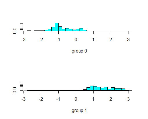
The below plot shows how the response class has been classified by the LDA classifier. The X-axis shows the value of line defined by the co-efficient of linear discriminant for LDA model. The two groups are the groups for response classes.

ldahist(predmodel.train.lda$x[,1], g= predmodel.train.lda$class)
       

 Now we will check for model accuracy for test data 0.7983
attach(test)
predmodel.test.lda = predict(lda.model, newdata=test)
table(Predicted=predmodel.test.lda$class, Survived=test$Survived)
         Survived
Predicted   0   1
        0 189  46
        1  26  96
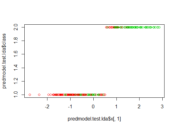
The below figure shows how the test data has been classified. The Predicted Group-1 and Group-2 has been colored with actual classification with red and green color. The mix of red and green color in the Group-1 and Group-2 shows the incorrect classification prediction.
par(mfrow=c(1,1))
plot(predmodel.test.lda$x[,1], predmodel.test.lda$class, col=test$Survived+10)


QDA Model

Next we will fit the model to QDA as below. The equation is same as LDA and it outputs the prior probabilities and Group means. Please note that 'prior probability' and 'Group Means' values are same as of LDA.
attach(train)
qda.model = qda (factor(Survived)~factor(Pclass)+Sex+Age+SibSp, data=train)
qda.model
> qda.model
Call:
qda(factor(Survived) ~ factor(Pclass) + Sex + Age + SibSp, data = train)

Prior probabilities of groups:
        0         1 
0.6254682 0.3745318 

Group means:
  factor(Pclass)2 factor(Pclass)3   Sexmale      Age     SibSp
0       0.1736527       0.6736527 0.8413174 30.27826 0.5538922
1       0.2200000       0.3750000 0.3100000 27.87822 0.4900000
In the next step, we will predict for training and test observation and check for their accuracy. Here training data accuracy: 0.8033 and testing accuracy is 0.7955.
##Predicting training results.
predmodel.train.qda = predict(qda.model, data=train)
table(Predicted=predmodel.train.qda$class, Survived=Survived)
         Survived
Predicted   0   1
        0 269  44
        1  65 156
##Predicting test results.
attach(test)
predmodel.test.qda = predict(qda.model, newdata=test)
table(Predicted=predmodel.test.qda$class, Survived=test$Survived)
         Survived
Predicted   0   1
        0 179  36
        1  36 106

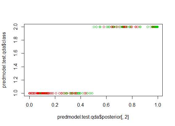
The below figure shows how the test data has been classified using the QDA model. The Predicted Group-1 and Group-2 has been colored with actual classification with red and green color. The mix of red and green color in the Group-1 and Group-2 shows the incorrect classification prediction.
par(mfrow=c(1,1))
plot(predmodel.test.qda$posterior[,2], predmodel.test.qda$class, col=test$Survived+10)


Conclusion

LDA and QDA work well when class separation and normality assumption holds true in the dataset. If the dataset is not normal then Logistic regression has an edge over LDA and QDA model. Logistic regression does not work properly if the response classes are fully separated from each other. In general, logistic regression is used for binomial classification and in case of multiple response classes, LDA and QDA are more popular.

Reference

    1. Statistics for Business By Robert Stine, Dean Foster 2. An Introduction to Statistical Learning, with Application in R. By James, G., Witten, D., Hastie, T., Tibshirani, R.
Share:

Linear Regression - Part 3

Machine Learning (ML) is a field of study that provides the capability to a Machine to understand data and to learn from the data. ML is not only about analytics modeling but it is end-to-end modeling that broadly involves following steps:
    - Defining problem statement 
     - Data collection. 
    - Exploring, Cleaning and transforming data. 
    - Making the analytics model. 
    - Dashboard creation & deployment of the model.
Machine learning has two distinct field of study - supervised learning and unsupervised learning. Supervised learning technique generates a response based on the set of input features. Unsupervised learning does not have any response variable and it explores the association and interaction between input features. In the following topic, I will discuss linear regression that is an example of supervised learning technique.

How to apply linear regression

The coefficient for linear regression is calculated based on the sample data. The basic assumption here is that the sample is not biased. This assumption makes sure that the sample does not necessarily always overestimate or underestimate the coefficients. The idea is that a particular sample may overestimate or underestimate but if one takes multiple samples and try to estimate the coefficient multiple times, then the average of co-efficient from multiple samples will be spot on.


Extract the data and create the training and testing sample

For the current model, let’s take the Boston dataset that is part of the MASS library in R Studio. Following are the features available in Boston dataset. The problem statement is to predict ‘medv’ based on the set of input features.
library(MASS)
library(ggplot2)
attach(Boston)
names(Boston)
 [1] "crim"    "zn"      "indus"   "chas"    "nox"     "rm"      "age"     "dis"     "rad"    
[10] "tax"     "ptratio" "black"   "lstat"   "medv"   

Split the sample data and make the model

Split the input data into training and evaluation set and make the model for the training dataset. It can be seen that training dataset has 404 observations and testing dataset has 102 observations based on 80-20 split.
##Sample the dataset. The return for this is row nos.
set.seed(1)
row.number <- sample(1:nrow(Boston), 0.8*nrow(Boston))
train = Boston[row.number,]
test = Boston[-row.number,]
dim(train)
dim(test)
[1] 404  14
[1] 102  14

Explore the response variable

Let's check for the distribution of response variable ‘medv’. The following figure shows the three distributions of ‘medv’ original, log transformation and square root transformation. We can see that both ‘log’ and ‘sqrt’ does a decent job to transform ‘medv’ distribution closer to normal. In the following model, I have selected ‘log’ transformation but it is also possible to try out ‘sqrt’ transformation.
##Explore the data.
ggplot(train, aes(medv)) + geom_density(fill="blue")
ggplot(train, aes(log(medv))) + geom_density(fill="blue")
ggplot(train, aes(sqrt(medv))) + geom_density(fill="blue")
        

Model Building – Model 1

Now as a first step we will fit the multiple regression models. We will start by taking all input variables in the multiple regression.
#Let’s make default model.
model1 = lm(log(medv)~., data=train)
summary(model1)
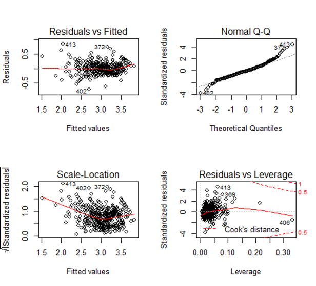
par(mfrow=c(2,2))
plot(model1)
Call:
lm(formula = log(medv) ~ ., data = train)

Residuals:
     Min       1Q   Median       3Q      Max 
-0.72354 -0.11993 -0.01279  0.10682  0.84791 

Coefficients:
              Estimate Std. Error t value Pr(>|t|)    
(Intercept)  4.2812343  0.2289799  18.697  < 2e-16 ***
crim        -0.0133166  0.0019722  -6.752 5.30e-11 ***
zn           0.0012855  0.0006558   1.960 0.050678 .  
indus        0.0032675  0.0029440   1.110 0.267724    
chas         0.1093931  0.0378934   2.887 0.004108 ** 
nox         -0.9457575  0.1748322  -5.410 1.10e-07 ***
rm           0.0651669  0.0186119   3.501 0.000516 ***
age          0.0010095  0.0006322   1.597 0.111139    
dis         -0.0475650  0.0092928  -5.119 4.85e-07 ***
rad          0.0176230  0.0030523   5.774 1.59e-08 ***
tax         -0.0006691  0.0001739  -3.847 0.000140 ***
ptratio     -0.0364731  0.0059456  -6.134 2.10e-09 ***
black        0.0003882  0.0001205   3.223 0.001377 ** 
lstat       -0.0310961  0.0022960 -13.543  < 2e-16 ***
---
Signif. codes:  0 ‘***’ 0.001 ‘**’ 0.01 ‘*’ 0.05 ‘.’ 0.1 ‘ ’ 1

Residual standard error: 0.195 on 390 degrees of freedom
Multiple R-squared:  0.7733, Adjusted R-squared:  0.7658 
F-statistic: 102.3 on 13 and 390 DF,  p-value: < 2.2e-16
                                      Is there a relationship between predictor and response variables? 
We can answer this using F stats. This defines the collective effect of all predictor variables on the response variable. In this model, F=102.3 is far greater than 1, and so it can be concluded that there is a relationship between predictor and response variable.

Which of the predictor variables are significant?
Based on the ‘p-value’ we can conclude on this. The lesser the ‘p’ value the more significant is the variable. From the ‘summary’ dump we can see that ‘zn’, ‘age’ and ‘indus’ are less significant features as the ‘p’ value is large for them. In next model, we can remove these variables from the model.

Is this model fit?
We can answer this based on R2 (multiple-R-squared) value as it indicates how much variation is captured by the model. R2 closer to 1 indicates that the model explains the large value of the variance of the model and hence a good fit. In this case, the value is 0.7733 (closer to 1) and hence the model is a good fit. Observation from the plot

Fitted vs Residual graph
Residuals plots should be random in nature and there should not be any pattern in the graph. The average of the residual plot should be close to zero. From the above plot, we can see that the red trend line is almost at zero except at the starting location.

Normal Q-Q Plot Q-Q plot
Itshows whether the residuals are normally distributed. Ideally, the plot should be on the dotted line. If the Q-Q plot is not on the line then models need to be reworked to make the residual normal. In the above plot, we see that most of the plots are on the line except at towards the end.

Scale-Location
This shows how the residuals are spread and whether the residuals have an equal variance or not.

Residuals vs Leverage
The plot helps to find influential observations. Here we need to check for points that are outside the dashed line. A point outside the dashed line will be influential point and removal of that will affect the regression coefficients.

Model Building - Model 2

As the next step, we can remove the four lesser significant features (‘zn’, age’ and ‘indus’ ) and check the model again.
# remove the less significant feature
model2 = update(model1, ~.-zn-indus-age) 
summary(model2) 
Call:
lm(formula = log(medv) ~ crim + chas + nox + rm + dis + rad + 
    tax + ptratio + black + lstat, data = train)

Residuals:
     Min       1Q   Median       3Q      Max 
-0.72053 -0.11852 -0.01833  0.10495  0.85353 

Coefficients:
              Estimate Std. Error t value Pr(>|t|)    
(Intercept)  4.2623092  0.2290865  18.606  < 2e-16 ***
crim        -0.0129937  0.0019640  -6.616 1.21e-10 ***
chas         0.1178952  0.0378684   3.113 0.001986 ** 
nox         -0.8549561  0.1627727  -5.252 2.46e-07 ***
rm           0.0731284  0.0180930   4.042 6.38e-05 ***
dis         -0.0465887  0.0073232  -6.362 5.55e-10 ***
rad          0.0157173  0.0028977   5.424 1.02e-07 ***
tax         -0.0005108  0.0001494  -3.418 0.000697 ***
ptratio     -0.0384253  0.0056084  -6.851 2.84e-11 ***
black        0.0003987  0.0001206   3.307 0.001031 ** 
lstat       -0.0295185  0.0021192 -13.929  < 2e-16 ***
---
Signif. codes:  0 ‘***’ 0.001 ‘**’ 0.01 ‘*’ 0.05 ‘.’ 0.1 ‘ ’ 1

Residual standard error: 0.1959 on 393 degrees of freedom
Multiple R-squared:  0.7696, Adjusted R-squared:  0.7637 
F-statistic: 131.2 on 10 and 393 DF,  p-value: < 2.2e-16

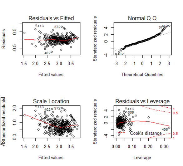
par(mfrow=c(2,2))
plot(model2)

         :
Is there a relationship between predictor and response variable? 
F=131.2 is far greater than 1 and this value is more than the F value of the previous model. It can be concluded that there is a relationship between predictor and response variable.

Which of the variable are significant? 
Now in this model, all the predictors are significant. Is this model fit? R2 =0.7696 is closer to 1 and so this model is a good fit. Please note that this value has decreased a little from the first model but this should be fine as removing three predictors caused a drop from 0.7733 to 0.7696 and this is a small drop. In other words, the contribution of three predictors towards explaining the variance is an only small value(0.0037) and hence it is better to drop the predictor.

Observation of the plot
All the four plots look similar to the previous model and we don’t see any major effect.

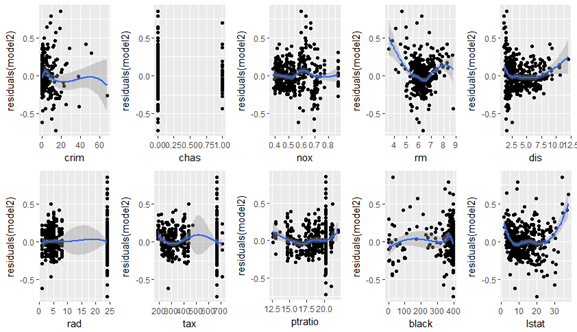
Check for predictor vs Residual Plot

In the next step, we will check the residual graph for all significant features from Model 2. We need to check if we see any pattern in the residual plot. Ideally, the residual plot should be random plot and we should not see a pattern. In the following plots, we can see some non-linear pattern for features like ‘crim’, ‘rm’, ‘nox’ etc.

##Plot the residual plot with all predictors.
attach(train)
require(gridExtra)
plot1 = ggplot(train, aes(crim, residuals(model2))) + geom_point() + geom_smooth()
plot2=ggplot(train, aes(chas, residuals(model2))) + geom_point() + geom_smooth()
plot3=ggplot(train, aes(nox, residuals(model2))) + geom_point() + geom_smooth()
plot4=ggplot(train, aes(rm, residuals(model2))) + geom_point() + geom_smooth()
plot5=ggplot(train, aes(dis, residuals(model2))) + geom_point() + geom_smooth()
plot6=ggplot(train, aes(rad, residuals(model2))) + geom_point() + geom_smooth()
plot7=ggplot(train, aes(tax, residuals(model2))) + geom_point() + geom_smooth()
plot8=ggplot(train, aes(ptratio, residuals(model2))) + geom_point() + geom_smooth()
plot9=ggplot(train, aes(black, residuals(model2))) + geom_point() + geom_smooth()
plot10=ggplot(train, aes(lstat, residuals(model2))) + geom_point() + geom_smooth()
grid.arrange(plot1,plot2,plot3,plot4,plot5,plot6,plot7,plot8,plot9,plot10,ncol=5,nrow=2)
            

Model Building - Model 3 & Model 4

We can now enhance the model by adding a square term to check for non-linearity. We can first try model3 by introducing square terms for all features ( from model 2). And in the next iteration, we can remove the insignificant feature from the model.
#Lets  make default model and add square term in the model.
model3 = lm(log(medv)~crim+chas+nox+rm+dis+rad+tax+ptratio+
black+lstat+ I(crim^2)+ I(chas^2)+I(nox^2)+ I(rm^2)+ I(dis^2)+ 
I(rad^2)+ I(tax^2)+ I(ptratio^2)+ I(black^2)+ I(lstat^2), data=train)
summary(model3)
Call:
lm(formula = log(medv) ~ crim + chas + nox + rm + dis + rad + tax + 
ptratio + black + lstat + I(crim^2) + I(chas^2) + I(nox^2) + 
I(rm^2) + I(dis^2) + I(rad^2) + I(tax^2) + I(ptratio^2) + 
I(black^2) + I(lstat^2), data = train)

Residuals:
     Min       1Q   Median       3Q      Max 
-0.78263 -0.09843 -0.00799  0.10008  0.76342 

Coefficients: (1 not defined because of singularities)
               Estimate Std. Error t value Pr(>|t|)    
(Intercept)   7.742e+00  9.621e-01   8.048 1.06e-14 ***
crim         -2.532e-02  5.203e-03  -4.866 1.66e-06 ***
chas          1.209e-01  3.481e-02   3.474 0.000572 ***
nox          -3.515e-01  1.136e+00  -0.309 0.757224    
rm           -6.061e-01  1.394e-01  -4.349 1.75e-05 ***
dis          -1.183e-01  2.563e-02  -4.615 5.36e-06 ***
rad           1.831e-02  9.843e-03   1.860 0.063675 .  
tax          -4.160e-04  5.687e-04  -0.731 0.464961    
ptratio      -1.783e-01  7.748e-02  -2.301 0.021909 *  
black         1.450e-03  5.379e-04   2.695 0.007340 ** 
lstat        -4.860e-02  6.009e-03  -8.088 8.05e-15 ***
I(crim^2)     1.542e-04  8.700e-05   1.773 0.077031 .  
I(chas^2)            NA         NA      NA       NA    
I(nox^2)     -5.801e-01  8.492e-01  -0.683 0.494947    
I(rm^2)       5.239e-02  1.100e-02   4.762 2.73e-06 ***
I(dis^2)      6.691e-03  2.077e-03   3.222 0.001383 ** 
I(rad^2)      8.069e-05  3.905e-04   0.207 0.836398    
I(tax^2)     -2.715e-07  6.946e-07  -0.391 0.696114    
I(ptratio^2)  4.174e-03  2.203e-03   1.895 0.058860 .  
I(black^2)   -2.664e-06  1.187e-06  -2.244 0.025383 *  
I(lstat^2)    5.741e-04  1.663e-04   3.451 0.000620 ***
---
Signif. codes:  0 ‘***’ 0.001 ‘**’ 0.01 ‘*’ 0.05 ‘.’ 0.1 ‘ ’ 1

Residual standard error: 0.1766 on 384 degrees of freedom
Multiple R-squared:  0.8169, Adjusted R-squared:  0.8079 
F-statistic: 90.19 on 19 and 384 DF,  p-value: |t|)    
##Removing the insignificant variables.
model4=update(model3, ~.-nox-rad-tax-I(crim^2)-I(chas^2)-I(rad^2)-
I(tax^2)-I(ptratio^2)-I(black^2))
summary(model4)
Call:
lm(formula = log(medv) ~ crim + chas + rm + dis + ptratio + black + 
    lstat + I(nox^2) + I(rm^2) + I(dis^2) + I(lstat^2), data = train)

Residuals:
     Min       1Q   Median       3Q      Max 
-0.73918 -0.09787 -0.00723  0.08868  0.82585 

(Intercept)  6.4071124  0.4571101  14.017  < 2e-16 ***
crim        -0.0125562  0.0016777  -7.484 4.78e-13 ***
chas         0.1353044  0.0356980   3.790 0.000174 ***
rm          -0.7248878  0.1428717  -5.074 6.04e-07 ***
dis         -0.0915153  0.0242616  -3.772 0.000187 ***
ptratio     -0.0247304  0.0050367  -4.910 1.34e-06 ***
black        0.0002375  0.0001134   2.094 0.036928 *  
lstat       -0.0461831  0.0061301  -7.534 3.44e-13 ***
I(nox^2)    -0.6335121  0.1185127  -5.346 1.53e-07 ***
I(rm^2)      0.0632918  0.0112473   5.627 3.49e-08 ***
I(dis^2)     0.0049036  0.0020706   2.368 0.018363 *  
I(lstat^2)   0.0004675  0.0001692   2.763 0.006003 ** 
---
Signif. codes:  0 ‘***’ 0.001 ‘**’ 0.01 ‘*’ 0.05 ‘.’ 0.1 ‘ ’ 1

Residual standard error: 0.1852 on 392 degrees of freedom
Multiple R-squared:  0.7946, Adjusted R-squared:  0.7888 
F-statistic: 137.9 on 11 and 392 DF,  p-value: < 2.2e-16 
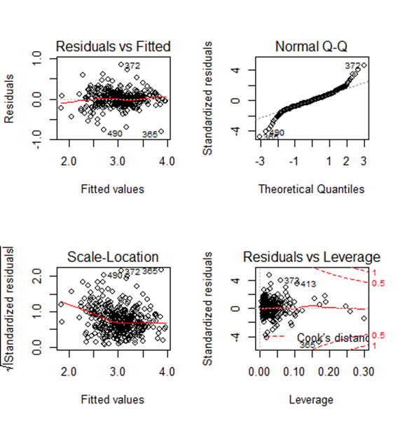
par(mfrow=c(2,2))
plot(model4)
     
Observation from summary (model4) Is there a relationship between predictor and response variables? F-Stat is 137.9 and it is far greater than 1. So there is a relationship between predictor and response variable. Which of the predictor variable are significant? All predictor variables are significant. Is this model fit? R2 is 0.7946 and this is more ( and better ) than our first and second model.

Prediction

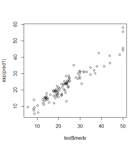
Till now we were checking training-error but the real goal of the model is to reduce the testing error. As we already split the sample dataset into training and testing dataset, we will use test dataset to evaluate the model that we have arrived upon. We will make a prediction based on ‘Model 4’ and will evaluate the model. As the last step, we will predict the ‘test’ observation and will see the comparison between predicted response and actual response value. RMSE explains on an average how much of the predicted value will be from the actual value. Based on RMSE = 3.278, we can conclude that on an average predicted value will be off by 3.278 from the actual value.
pred1 <- predict(model4, newdata = test)
rmse <- sqrt(sum((exp(pred1) - test$medv)^2)/length(test$medv))
c(RMSE = rmse, R2=summary(model4)$r.squared)
          RMSE        R2 
3.2782608 0.7946003 
par(mfrow=c(1,1))
plot(test$medv, exp(pred1))
             

Conclusion

The example shows how to approach linear regression modeling. The model that is created still has scope for improvement as we can apply techniques like Outlier detection, Correlation detection to further improve the accuracy of more accurate prediction. One can as well use an advanced technique like Random Forest and Boosting technique to check whether the accuracy can be further improved for the model. A piece of warning is that we should refrain from overfitting the model for training data as the test accuracy of the model will reduce for test data in case of overfitting.

Reference

    1. Statistics for Business By Robert Stine, Dean Foster 2. An Introduction to Statistical Learning, with Application in R. By James, G., Witten, D., Hastie, T., Tibshirani, R.
Share:

Wednesday, 6 May 2020

Linear Regression - Part 2


In the previous post we discussed how to calculate the coefficient for simple and multiple regression.
In this post we will study how to check the accuracy of the coefficient values and how to evaluate the model fit.

Assumptions

Before jumping into the coefficient accuracy, let's list down the assumption that we make to calculate the coefficient :
- The sample taken to calculate the coefficient is unbiased.
- This means that model does not overestimate or underestimate the coefficient. So for a particular  sample, model may overestimate or underestimate the coefficient but if  multiple samples are taken then average value of coefficients calculated over multiple sample will be spot on.

Standard Error of coefficients

Standard error defines the sample to sample variability of β0 and β1. It can also be defined as the average value by which the coefficient will differ from TRUE value. Following are the standard error for β0 and β1.


From the above equation we can note that :
- The more the 'X' value is spread, the lower will be the standard error because of denominator in SE(β0).
- The more the 'Y' value is spread, the higher will be the standard error.

The following diagram depicts the behavior that the more X value is spread the more the line will be closer to each other and hence lower will be standard error.

More variation (spread) is 'X" results in better estimate of slope β1.
Based on the standard error, that is calculate above, we can also define the range of coefficient with 95% confidence interval :

Confidence interval of β1 
   [ β1 + 2SE(β1) , β1 - 2SE(β1) ]
Confidence interval of β0 
  [ β0 + 2SE(β0) , β0 - 2SE(β0) ]

In simple words it defines that if we change the sample and then calculate the coefficient again then 95% of time the coefficient of βand β0  will fall in the range of confidence interval as explained above. 

Check for NULL Hypothesis

To find the relation between coefficient and response variable, we need to check that coefficients are sufficiently far from zero value.

How far from zero ?

      t = (β1 - 0) / SE(β1)

The larger the 't' value, the more will be the confidence that coefficient is far from 0. If 't' value is greater than 2 then we can say that '0' value is outside the range of 95% confidence interval for coefficient. In other words if we change the sample and again calculate β1  then 95% of times βvalue will not be 0 or outside the range of 0. Note that if βis equal to zero then it means that there is no association between corresponding input and response variable.

Importance of a input variable:
t-stat and corresponding p-stat  provides the details about importance of a particular variable. The higher the t-stat, the lower will be the p-stat and hence higher will be the importance of the variable. When doing Regression, we need to check which variable is not important(lower t value and so higher p-value) and based on that we can remove corresponding variable from the model.

Model Accuracy

Quality of linear regression model fit is accessed using following :

RSE : It is average amount by which the predicted value will deviate from true regression line. RSE provides the lack of fit of the model. One drawback of RSE is that it provides the o/p in the unit of the response variable and hence it is difficult to device any standard to find whether RSE is more or less. 

R2 - ( R-squared ) -  R2 is similar to RSE except that it takes care of the drawback of RSE. It is of the form of proportion so that its value will always be in the range 0 to 1 with '0' means that model is not good fit and '1' means that model is good fit. 


Why we need to check t-stat and R2  ?

Note than R2 can't be only measure to check the statistical significance of the model as R2 increases with the increase of number of input variables or predictors. That's why we need to check the t-stat of every input variable to check its statistical significance of corresponding input variable.

Summary

         In this article we saw various measures to check the standard error of coefficient and how to evaluate the regression model. We also saw how to check the importance of a particular input variable and how to include or exclude them from the model. In the next article we will write R code for regression and explain the model based on the various parameters provided by the mode.


Share:

Saturday, 2 May 2020

Linear Regression - Part 1


Introduction

Linear Regression is supervised learning techinique to model the quantitative data. The model fits a line that is closest to all observation points. The basic assumption here is that functional form is the line and it is possible to fit the line that will be closest to all observation. Because of its simplicity, LR serves as good starting point to provide benchmark on which more complex models can be built.

Following figure shows a 2-dimensional X-Y plot  and the corresponding line that fits between points so that the line is closest to all point.

Regression Line

Basic maths on how to draw a line in two dimension.

Let's start with basic on what parameters are required to draw a line in two dimension plane. From the following figure, it is easy to figure out that intercept (β0 and slope (β1 parameters are required to draw the line. 
  • Intercept - Intercept define the Y value when input X =0.
  • Slope - Slope defines the angle by which line can be rotated across the intercept.
Intercept (β0) and Slope on a line (β1).

If we change either of them, the position or orientation of the line will change resulting in new line. 

As shown in the following 3-d figure, the understanding of 2-dimension can be extended to higher dimension as well to draw a line. For example in 3 dimension, with one output variable (Z) and two input variable ( X and Y),  three parameters, one intercept (β0) and two slopes (β1, β2), are required to draw a line.

Intercept (β0) and Slope(β1, β2 ) on a 3-d line .


Basic Maths for Linear Regression.

Mathematically, linear regression equation can be written as one of the following two ways depending on number of input variable.

Simple Regression

Simple regression has one input variable (Predictor) and one output variable (Response variable). In the following equation, X defines the inputs feature and Y defines the output variable.

Multiple Regression

Multiple regression has more than one input variable (Predictor) and one output variable (Response variable). In the following equation X = (x1, x2.. xn) defines the input variable and Y defines the output variable.


The simple and multiple regression technique allows us to estimate the coefficient (β1, β2...βn) of the line depending on the sample dataset provided. This allows us to estimate the line so that it is nearest to all sample point collectively.

How to estimate the co-efficient ?

Coefficient estimates are done in two steps:
  • Estimate the error - This define the error between actual and predicted value for each observation.
  • Minimize the error - There are various ways to minimize the error but LEAST SQUARE is most popular among them. As the names implies, least square minimizes the error after taking the square of prediction error for every observation.

Step-1 : Estimate the error 

Estimation error can be calculated by the difference between actual value and predicted value. From the following figure, we can see that error (e9) is defined by difference between actual-value and predicted value for observation#9.
Error estimation
Based on the above understanding, it is possible to calculate the the error for each individual observation in the model.
For a sample having 'n' observation error for individual observation will be = [e1 , e2e3e4e5, ...... , en]

Step-2: Minimize the error 


Now that we found observation error, the next step is to minimize the total error in the model. For this first residual sum of errors (RSS) is calculated and then total error (RSS) is minimized to get the coefficient of intercept and slope. This is also done in two steps:

Calculate Residual Sum of Squares(RSS) and differentiate - Calculate total sum of square of errors. Note that errors are squared so that we get absolute errors and total errors equation can be differentiated to get the coefficient for intercept and slope for least error line. 
                       
                       RSS = e1^2+e2^2+e3^2+⋯+ en^2

                       RSS = (y101x1)2+ (y2-β02x2)2 +…. + (yn0nxn)2

The coefficients are calculated as below :


where 


How to interpret the co-efficient?


Simple Regression

Suppose we want to predict Y(=Sales) of the product based on the input X( = TV budget ) and the co-efficient for  for β0  and β1 are calculated as below :

        
  • β1 = 0.0475 -  Average increase of Y=Sales associated with one unit increase in X=TV Budget. We can conclude that for additional increase in TV budget of 1000 unit, Sales will increase by 47.5
  • β0= 7.03 - Expected value of Y=Sales when X = TV Budget is equal to 0. We can conclude that If TV budget is 0, then default sales will be 7.03 unit.

Multiple Regression

Suppose we want to predict Y(=Sales) of the product based on the three input X1(TV budget ), X2(Radio Budget), and X3(Newspaper Budget) and the corresponding co-efficient are  β0 , β1,  β2 and β3 are calculated as below :

        
  • β1 = 0.046 -  Average increase of Y=Sales associated with one unit increase in X=TV Budget, provided that there is no increase in budget of other predictors (Radio and Newspaper). We can conclude that for additional increase in TV budget of 1000 unit, provided that all other budgets are constant, Sales will increase by 46 units.
  • β0= 0.0475 - Expected value of Y=Sales when there has been no budgetary expenditure on TV, Radio and Newspaper.  In this case we can conclude that default sales will be 2.939 unit.


Summary

In this blog i presented you the basic concept on Regression and how to calculate the LEAST ERROR line by estimating the corresponding co-efficient for intercept and slope. In the next blog, i will explain about how to calculate errors in the intercept and slope coefficient and Regression model. I will also present a use case to show how to different the various parameters to evaluate the model.


Share:

Feature Top (Full Width)

Pageviews

Search This Blog

Blogs