


Principal Component Analysis (PCA) is unsupervised learning technique and it is used to reduce the dimension of the data with minimum loss of information. PCA is used in an application like face recognition and image compression.
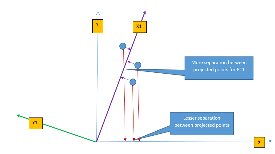
PCA transforms the feature from original space to a new feature space to increase the separation between data. The following figure shows the projection of three points on X-axis and X1-axis. It is easy to understand that projected points on X1-axis are better(more) separated than projected points on X-axis This is because the X1-axis is drawn in the direction of the highest variance of data points and so the projection of a point on this line results in maximum separation. PCA identifies the direction where the perpendicular distance from the data-point to the ‘maximum variance direction’ is smallest and projection of data on this line yields maximum separation.

The above equation transforms the 'p' input feature X using co-efficient ϕ to Z. Please note that the transformed variable Z is a linear combination of ‘all’ input features X1, X2...Xp and none of the input features are discarded. The above equation can be extended to multiple dimension to create multiple transformed variable Z1, Z2, … Zm using a different set of a coefficient. Transformed variables Z1, Z2, … Zm will then be used for model building and if m<p then overall result will be a reduction in dimension from p to m.
Intuitively we can think of transformation as rotating the axis and taking the projection of data points. From the figure above, we can perform the linear transformation of data points by changing the axis from X to X1 and take the projection of data-points on X1-axis.
PCA changes the axis towards the direction of maximum variance and then takes projection on this new axis. The direction of maximum variance is represented by Principal Components (PC1). There are multiple principal components depending on the number of dimensions (features) in the dataset and they are orthogonal to each other. The maximum number of principal component is same as a number of dimension of data. For example, in the above figure, for two-dimension data, there will be max of two principal components (PC1 & PC2). The first principal component defines the most of the variance, followed by second principal component, third principal component and so on. Dimension reduction comes from the fact that it is possible to discard last few principal components as they will not capture much variance in the data. Following steps shows how to get the principal components:
We will use
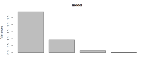
The following plots show the dominance of PC1. The bar graph shows the proportion of variance explained by principal components. We can see that PC1 explains 72% of the variance, PC2 explains 23% of the variance and so on. The same has been shown in the plot below. Please note that PC1 and PC2 together explain around 95% of the variance and we can discard the PC3 and PC4 because their contribution towards explaining the variance is just 5%.
Linear transformation, Dimension reduction & PCA
Z =∑{j=1}p ϕj * XjThe above equation transforms the 'p' input feature X using co-efficient ϕ to Z. Please note that the transformed variable Z is a linear combination of ‘all’ input features X1, X2...Xp and none of the input features are discarded. The above equation can be extended to multiple dimension to create multiple transformed variable Z1, Z2, … Zm using a different set of a coefficient. Transformed variables Z1, Z2, … Zm will then be used for model building and if m<p then overall result will be a reduction in dimension from p to m.
Intuitively we can think of transformation as rotating the axis and taking the projection of data points. From the figure above, we can perform the linear transformation of data points by changing the axis from X to X1 and take the projection of data-points on X1-axis.
PCA changes the axis towards the direction of maximum variance and then takes projection on this new axis. The direction of maximum variance is represented by Principal Components (PC1). There are multiple principal components depending on the number of dimensions (features) in the dataset and they are orthogonal to each other. The maximum number of principal component is same as a number of dimension of data. For example, in the above figure, for two-dimension data, there will be max of two principal components (PC1 & PC2). The first principal component defines the most of the variance, followed by second principal component, third principal component and so on. Dimension reduction comes from the fact that it is possible to discard last few principal components as they will not capture much variance in the data. Following steps shows how to get the principal components:
- Find the mean of each feature and then subtract observations from the mean for each of the features so that the origin is changed to the centroid. This is done to ensure that PC1 will pass through centroid origin, otherwise PC1 will still pass through centroid but this will not be the centroid. Please read through the reference [2] for more details.
- Find the covariance matrix. This defines the correlation between different features in matrix form.
- Then find the eigenvector and eigenvalue for the covariance matrix obtained in the previous step. Eigenvalues defines length of the eigenvector or the contribution of each principal component to defining the variance of the dataset.
How to implement PCA in R
We will use the famous ‘iris’ data for PCA. This dataset has 4 numerical features and 1 categorical feature.input = read.csv("iris.csv")
names(input)
str(input)
> names(input)
[1] "sepal_len" "sepal_wid" "petal_len" "petal_wid" "class"
> str(input)
'data.frame': 150 obs. of 5 variables:
$ sepal_len: num 5.1 4.9 4.7 4.6 5 5.4 4.6 5 4.4 4.9 ...
$ sepal_wid: num 3.5 3 3.2 3.1 3.6 3.9 3.4 3.4 2.9 3.1 ...
$ petal_len: num 1.4 1.4 1.3 1.5 1.4 1.7 1.4 1.5 1.4 1.5 ...
$ petal_wid: num 0.2 0.2 0.2 0.2 0.2 0.4 0.3 0.2 0.2 0.1 ...
$ class : Factor w/ 3 levels "Iris-setosa",..: 1 1 1 1 1 1 1 1 1 1 ..
We will use
prcomp function for PCA. The prcomp provides four output as dumped below.
- Sdev – This defines the standard deviation of projected points on PC1, PC2, PC3 and PC3. As expected, the standard deviation of projected point is in decreasing order from PC1 to PC4.
- Rotation – This defines the principal components axis. Here there are four principal components as there are four input features.
- Center/Scale – These are mean and standard deviation of input features in original feature space (without any transformation).
model = prcomp(input[,1:4], scale=TRUE)
model$sdev
model$rotation
model$center
model$scale
model$sdev
[1] 1.7061120 0.9598025 0.3838662 0.1435538
> model$rotation
                 PC1         PC2        PC3        PC4
sepal_len  0.5223716 -0.37231836  0.7210168  0.2619956
sepal_wid -0.2633549 -0.92555649 -0.2420329 -0.1241348
petal_len  0.5812540 -0.02109478 -0.1408923 -0.8011543
petal_wid  0.5656110 -0.06541577 -0.6338014  0.5235463
> model$center
sepal_len sepal_wid petal_len petal_wid
 5.843333  3.054000  3.758667  1.198667
> model$scale
sepal_len sepal_wid petal_len petal_wid
0.8280661 0.4335943 1.7644204 0.7631607
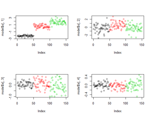
The following figure shows the plots of projected points on principal components. It is very clear that projected points on PC1 clearly classify the data but the plots of projected points by lower principal components (for PC2, PC3 & PC4) is not able to classify the data as convincingly as PC1.
par(mfrow=c(2,2))
plot(model$x[,1], col=input[,5])
plot(model$x[,2], col=input[,5])
plot(model$x[,3], col=input[,5])
plot(model$x[,4], col=input[,5])
The following plots show the dominance of PC1. The bar graph shows the proportion of variance explained by principal components. We can see that PC1 explains 72% of the variance, PC2 explains 23% of the variance and so on. The same has been shown in the plot below. Please note that PC1 and PC2 together explain around 95% of the variance and we can discard the PC3 and PC4 because their contribution towards explaining the variance is just 5%.
model$sdev^2 / sum(model$sdev^2)
plot(model)
> model$sdev^2 / sum(model$sdev^2)
[1] 0.727704521 0.230305233 0.036838320 0.005151927

PCA without ‘prcomp’
The following code shows how to get the direction on principal components using eigenvector. Please note that eigenvector is same as the output ofmodel$rotation using prcomp (in the previous example).
## Normalize the input feature.
input$sepal_len1 = (input$sepal_len - mean(input$sepal_len) )/sd(input$sepal_len)
input$sepal_wid1 = (input$sepal_wid - mean(input$sepal_wid))/sd(input$sepal_wid)
input$petal_len1 = (input$petal_len - mean(input$petal_len))/sd(input$petal_len)
input$petal_wid1 = (input$petal_wid - mean(input$petal_wid))/sd(input$petal_wid)

##Get the covarience matrix and eigen vector.
matrix_form = matrix(c(input$sepal_len1, input$sepal_wid1, input$petal_len1, input$petal_wid1), ncol=4)
m = cov(matrix_form)
eigenV = eigen(m)
eigenV$vectors
       [,1]        [,2]       [,3]       [,4]
[1,]  0.5223716 -0.37231836  0.7210168  0.2619956
[2,] -0.2633549 -0.92555649 -0.2420329 -0.1241348
[3,]  0.5812540 -0.02109478 -0.1408923 -0.8011543
[4,]  0.5656110 -0.06541577 -0.6338014  0.5235463
Conclusion
PCA is very useful in reducing the dimension of data. Some important point to note before using PCA:- As PCA tries to find the linear combination of data and if the data in the dataset has non-linear relation then PCA will not work efficiently.
- Data should be normalized before performing PCA. PCA is sensitive to scaling of data as higher variance data will drive the principal component.
Reference
- 1. An Introduction to Statistical Learning, with Application in R. By James, G., Witten, D., Hastie, T., Tibshirani, R.
- 2. How does centering the data get rid of the intercept in regression and PCA?


0 comments:
Post a Comment