Machine Learning (ML) is a field of study that provides the capability to a Machine to understand data and to learn from the data. ML is not only about analytics modeling but it is end-to-end modeling that broadly involves following steps:
 Is there a relationship between predictor and response variables?
We can answer this using F stats. This defines the collective effect of all predictor variables on the response variable. In this model, F=102.3 is far greater than 1, and so it can be concluded that there is a relationship between predictor and response variable.
Which of the predictor variables are significant?
Based on the ‘p-value’ we can conclude on this. The lesser the ‘p’ value the more significant is the variable. From the ‘summary’ dump we can see that ‘zn’, ‘age’ and ‘indus’ are less significant features as the ‘p’ value is large for them. In next model, we can remove these variables from the model.
Is this model fit?
We can answer this based on R2 (multiple-R-squared) value as it indicates how much variation is captured by the model. R2 closer to 1 indicates that the model explains the large value of the variance of the model and hence a good fit. In this case, the value is 0.7733 (closer to 1) and hence the model is a good fit. Observation from the plot
Fitted vs Residual graph
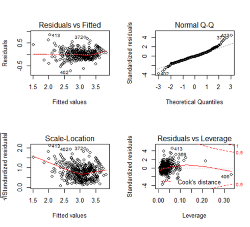
Residuals plots should be random in nature and there should not be any pattern in the graph. The average of the residual plot should be close to zero. From the above plot, we can see that the red trend line is almost at zero except at the starting location.
Normal Q-Q Plot Q-Q plot
Itshows whether the residuals are normally distributed. Ideally, the plot should be on the dotted line. If the Q-Q plot is not on the line then models need to be reworked to make the residual normal. In the above plot, we see that most of the plots are on the line except at towards the end.
Scale-Location
This shows how the residuals are spread and whether the residuals have an equal variance or not.
Residuals vs Leverage
The plot helps to find influential observations. Here we need to check for points that are outside the dashed line. A point outside the dashed line will be influential point and removal of that will affect the regression coefficients.
:
Is there a relationship between predictor and response variable?
F=131.2 is far greater than 1 and this value is more than the F value of the previous model. It can be concluded that there is a relationship between predictor and response variable.
Which of the variable are significant?
Now in this model, all the predictors are significant. Is this model fit? R2 =0.7696 is closer to 1 and so this model is a good fit. Please note that this value has decreased a little from the first model but this should be fine as removing three predictors caused a drop from 0.7733 to 0.7696 and this is a small drop. In other words, the contribution of three predictors towards explaining the variance is an only small value(0.0037) and hence it is better to drop the predictor.
Observation of the plot
All the four plots look similar to the previous model and we don’t see any major effect.

Observation from summary (model4) Is there a relationship between predictor and response variables? F-Stat is 137.9 and it is far greater than 1. So there is a relationship between predictor and response variable. Which of the predictor variable are significant? All predictor variables are significant. Is this model fit? R2 is 0.7946 and this is more ( and better ) than our first and second model.
- - Defining problem statement
- - Data collection.
- - Exploring, Cleaning and transforming data.
- - Making the analytics model.
- - Dashboard creation & deployment of the model.
How to apply linear regression
The coefficient for linear regression is calculated based on the sample data. The basic assumption here is that the sample is not biased. This assumption makes sure that the sample does not necessarily always overestimate or underestimate the coefficients. The idea is that a particular sample may overestimate or underestimate but if one takes multiple samples and try to estimate the coefficient multiple times, then the average of co-efficient from multiple samples will be spot on.Extract the data and create the training and testing sample
For the current model, let’s take the Boston dataset that is part of the MASS library in R Studio. Following are the features available in Boston dataset. The problem statement is to predict ‘medv’ based on the set of input features.library(MASS) library(ggplot2) attach(Boston) names(Boston) [1] "crim" "zn" "indus" "chas" "nox" "rm" "age" "dis" "rad" [10] "tax" "ptratio" "black" "lstat" "medv"
Split the sample data and make the model
Split the input data into training and evaluation set and make the model for the training dataset. It can be seen that training dataset has 404 observations and testing dataset has 102 observations based on 80-20 split.##Sample the dataset. The return for this is row nos. set.seed(1) row.number <- sample(1:nrow(Boston), 0.8*nrow(Boston)) train = Boston[row.number,] test = Boston[-row.number,] dim(train) dim(test) [1] 404 14 [1] 102 14
Explore the response variable
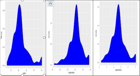
Let's check for the distribution of response variable ‘medv’. The following figure shows the three distributions of ‘medv’ original, log transformation and square root transformation. We can see that both ‘log’ and ‘sqrt’ does a decent job to transform ‘medv’ distribution closer to normal. In the following model, I have selected ‘log’ transformation but it is also possible to try out ‘sqrt’ transformation.##Explore the data. ggplot(train, aes(medv)) + geom_density(fill="blue") ggplot(train, aes(log(medv))) + geom_density(fill="blue") ggplot(train, aes(sqrt(medv))) + geom_density(fill="blue")

Model Building – Model 1
Now as a first step we will fit the multiple regression models. We will start by taking all input variables in the multiple regression.#Let’s make default model.
model1 = lm(log(medv)~., data=train)
summary(model1)
par(mfrow=c(2,2))
plot(model1)
Call:
lm(formula = log(medv) ~ ., data = train)
Residuals:
Min 1Q Median 3Q Max
-0.72354 -0.11993 -0.01279 0.10682 0.84791
Coefficients:
Estimate Std. Error t value Pr(>|t|)
(Intercept) 4.2812343 0.2289799 18.697 < 2e-16 ***
crim -0.0133166 0.0019722 -6.752 5.30e-11 ***
zn 0.0012855 0.0006558 1.960 0.050678 .
indus 0.0032675 0.0029440 1.110 0.267724
chas 0.1093931 0.0378934 2.887 0.004108 **
nox -0.9457575 0.1748322 -5.410 1.10e-07 ***
rm 0.0651669 0.0186119 3.501 0.000516 ***
age 0.0010095 0.0006322 1.597 0.111139
dis -0.0475650 0.0092928 -5.119 4.85e-07 ***
rad 0.0176230 0.0030523 5.774 1.59e-08 ***
tax -0.0006691 0.0001739 -3.847 0.000140 ***
ptratio -0.0364731 0.0059456 -6.134 2.10e-09 ***
black 0.0003882 0.0001205 3.223 0.001377 **
lstat -0.0310961 0.0022960 -13.543 < 2e-16 ***
---
Signif. codes: 0 ‘***’ 0.001 ‘**’ 0.01 ‘*’ 0.05 ‘.’ 0.1 ‘ ’ 1
Residual standard error: 0.195 on 390 degrees of freedom
Multiple R-squared: 0.7733, Adjusted R-squared: 0.7658
F-statistic: 102.3 on 13 and 390 DF, p-value: < 2.2e-16
 Is there a relationship between predictor and response variables?
 We can answer this using F stats. This defines the collective effect of all predictor variables on the response variable. In this model, F=102.3 is far greater than 1, and so it can be concluded that there is a relationship between predictor and response variable.
Which of the predictor variables are significant?
Based on the ‘p-value’ we can conclude on this. The lesser the ‘p’ value the more significant is the variable. From the ‘summary’ dump we can see that ‘zn’, ‘age’ and ‘indus’ are less significant features as the ‘p’ value is large for them. In next model, we can remove these variables from the model.
Is this model fit?
We can answer this based on R2 (multiple-R-squared) value as it indicates how much variation is captured by the model. R2 closer to 1 indicates that the model explains the large value of the variance of the model and hence a good fit. In this case, the value is 0.7733 (closer to 1) and hence the model is a good fit. Observation from the plot
Fitted vs Residual graph
Residuals plots should be random in nature and there should not be any pattern in the graph. The average of the residual plot should be close to zero. From the above plot, we can see that the red trend line is almost at zero except at the starting location.
Normal Q-Q Plot Q-Q plot
Itshows whether the residuals are normally distributed. Ideally, the plot should be on the dotted line. If the Q-Q plot is not on the line then models need to be reworked to make the residual normal. In the above plot, we see that most of the plots are on the line except at towards the end.
Scale-Location
This shows how the residuals are spread and whether the residuals have an equal variance or not.
Residuals vs Leverage
The plot helps to find influential observations. Here we need to check for points that are outside the dashed line. A point outside the dashed line will be influential point and removal of that will affect the regression coefficients.
Model Building - Model 2
As the next step, we can remove the four lesser significant features (‘zn’, age’ and ‘indus’ ) and check the model again.# remove the less significant feature
model2 = update(model1, ~.-zn-indus-age)
summary(model2)
Call:
lm(formula = log(medv) ~ crim + chas + nox + rm + dis + rad +
tax + ptratio + black + lstat, data = train)
Residuals:
Min 1Q Median 3Q Max
-0.72053 -0.11852 -0.01833 0.10495 0.85353
Coefficients:
Estimate Std. Error t value Pr(>|t|)
(Intercept) 4.2623092 0.2290865 18.606 < 2e-16 ***
crim -0.0129937 0.0019640 -6.616 1.21e-10 ***
chas 0.1178952 0.0378684 3.113 0.001986 **
nox -0.8549561 0.1627727 -5.252 2.46e-07 ***
rm 0.0731284 0.0180930 4.042 6.38e-05 ***
dis -0.0465887 0.0073232 -6.362 5.55e-10 ***
rad 0.0157173 0.0028977 5.424 1.02e-07 ***
tax -0.0005108 0.0001494 -3.418 0.000697 ***
ptratio -0.0384253 0.0056084 -6.851 2.84e-11 ***
black 0.0003987 0.0001206 3.307 0.001031 **
lstat -0.0295185 0.0021192 -13.929 < 2e-16 ***
---
Signif. codes: 0 ‘***’ 0.001 ‘**’ 0.01 ‘*’ 0.05 ‘.’ 0.1 ‘ ’ 1
Residual standard error: 0.1959 on 393 degrees of freedom
Multiple R-squared: 0.7696, Adjusted R-squared: 0.7637
F-statistic: 131.2 on 10 and 393 DF, p-value: < 2.2e-16
par(mfrow=c(2,2))
plot(model2)
:

Is there a relationship between predictor and response variable?
F=131.2 is far greater than 1 and this value is more than the F value of the previous model. It can be concluded that there is a relationship between predictor and response variable.
Which of the variable are significant?
Now in this model, all the predictors are significant. Is this model fit? R2 =0.7696 is closer to 1 and so this model is a good fit. Please note that this value has decreased a little from the first model but this should be fine as removing three predictors caused a drop from 0.7733 to 0.7696 and this is a small drop. In other words, the contribution of three predictors towards explaining the variance is an only small value(0.0037) and hence it is better to drop the predictor.
Observation of the plot
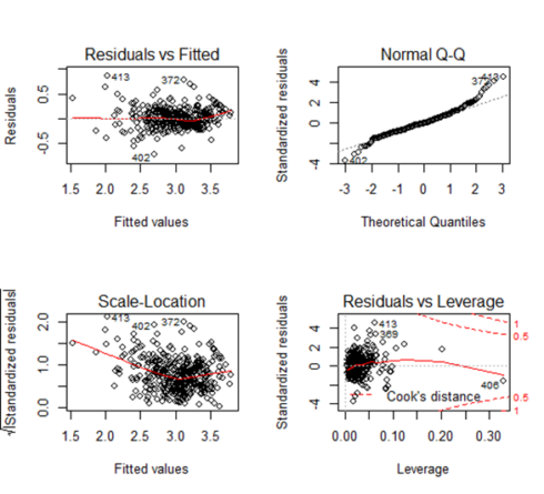
All the four plots look similar to the previous model and we don’t see any major effect.
Check for predictor vs Residual Plot
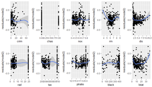
In the next step, we will check the residual graph for all significant features from Model 2. We need to check if we see any pattern in the residual plot. Ideally, the residual plot should be random plot and we should not see a pattern. In the following plots, we can see some non-linear pattern for features like ‘crim’, ‘rm’, ‘nox’ etc.##Plot the residual plot with all predictors. attach(train) require(gridExtra) plot1 = ggplot(train, aes(crim, residuals(model2))) + geom_point() + geom_smooth() plot2=ggplot(train, aes(chas, residuals(model2))) + geom_point() + geom_smooth() plot3=ggplot(train, aes(nox, residuals(model2))) + geom_point() + geom_smooth() plot4=ggplot(train, aes(rm, residuals(model2))) + geom_point() + geom_smooth() plot5=ggplot(train, aes(dis, residuals(model2))) + geom_point() + geom_smooth() plot6=ggplot(train, aes(rad, residuals(model2))) + geom_point() + geom_smooth() plot7=ggplot(train, aes(tax, residuals(model2))) + geom_point() + geom_smooth() plot8=ggplot(train, aes(ptratio, residuals(model2))) + geom_point() + geom_smooth() plot9=ggplot(train, aes(black, residuals(model2))) + geom_point() + geom_smooth() plot10=ggplot(train, aes(lstat, residuals(model2))) + geom_point() + geom_smooth() grid.arrange(plot1,plot2,plot3,plot4,plot5,plot6,plot7,plot8,plot9,plot10,ncol=5,nrow=2)

Model Building - Model 3 & Model 4
We can now enhance the model by adding a square term to check for non-linearity. We can first try model3 by introducing square terms for all features ( from model 2). And in the next iteration, we can remove the insignificant feature from the model.#Lets make default model and add square term in the model.
model3 = lm(log(medv)~crim+chas+nox+rm+dis+rad+tax+ptratio+
black+lstat+ I(crim^2)+ I(chas^2)+I(nox^2)+ I(rm^2)+ I(dis^2)+
I(rad^2)+ I(tax^2)+ I(ptratio^2)+ I(black^2)+ I(lstat^2), data=train)
summary(model3)
Call:
lm(formula = log(medv) ~ crim + chas + nox + rm + dis + rad + tax +
ptratio + black + lstat + I(crim^2) + I(chas^2) + I(nox^2) +
I(rm^2) + I(dis^2) + I(rad^2) + I(tax^2) + I(ptratio^2) +
I(black^2) + I(lstat^2), data = train)
Residuals:
Min 1Q Median 3Q Max
-0.78263 -0.09843 -0.00799 0.10008 0.76342
Coefficients: (1 not defined because of singularities)
Estimate Std. Error t value Pr(>|t|)
(Intercept) 7.742e+00 9.621e-01 8.048 1.06e-14 ***
crim -2.532e-02 5.203e-03 -4.866 1.66e-06 ***
chas 1.209e-01 3.481e-02 3.474 0.000572 ***
nox -3.515e-01 1.136e+00 -0.309 0.757224
rm -6.061e-01 1.394e-01 -4.349 1.75e-05 ***
dis -1.183e-01 2.563e-02 -4.615 5.36e-06 ***
rad 1.831e-02 9.843e-03 1.860 0.063675 .
tax -4.160e-04 5.687e-04 -0.731 0.464961
ptratio -1.783e-01 7.748e-02 -2.301 0.021909 *
black 1.450e-03 5.379e-04 2.695 0.007340 **
lstat -4.860e-02 6.009e-03 -8.088 8.05e-15 ***
I(crim^2) 1.542e-04 8.700e-05 1.773 0.077031 .
I(chas^2) NA NA NA NA
I(nox^2) -5.801e-01 8.492e-01 -0.683 0.494947
I(rm^2) 5.239e-02 1.100e-02 4.762 2.73e-06 ***
I(dis^2) 6.691e-03 2.077e-03 3.222 0.001383 **
I(rad^2) 8.069e-05 3.905e-04 0.207 0.836398
I(tax^2) -2.715e-07 6.946e-07 -0.391 0.696114
I(ptratio^2) 4.174e-03 2.203e-03 1.895 0.058860 .
I(black^2) -2.664e-06 1.187e-06 -2.244 0.025383 *
I(lstat^2) 5.741e-04 1.663e-04 3.451 0.000620 ***
---
Signif. codes: 0 ‘***’ 0.001 ‘**’ 0.01 ‘*’ 0.05 ‘.’ 0.1 ‘ ’ 1
Residual standard error: 0.1766 on 384 degrees of freedom
Multiple R-squared: 0.8169, Adjusted R-squared: 0.8079
F-statistic: 90.19 on 19 and 384 DF, p-value: |t|)
##Removing the insignificant variables.
model4=update(model3, ~.-nox-rad-tax-I(crim^2)-I(chas^2)-I(rad^2)-
I(tax^2)-I(ptratio^2)-I(black^2))
summary(model4)
Call:
lm(formula = log(medv) ~ crim + chas + rm + dis + ptratio + black +
    lstat + I(nox^2) + I(rm^2) + I(dis^2) + I(lstat^2), data = train)

Residuals:
     Min       1Q   Median       3Q      Max
-0.73918 -0.09787 -0.00723  0.08868  0.82585

(Intercept)  6.4071124  0.4571101  14.017  < 2e-16 ***
crim        -0.0125562  0.0016777  -7.484 4.78e-13 ***
chas         0.1353044  0.0356980   3.790 0.000174 ***
rm          -0.7248878  0.1428717  -5.074 6.04e-07 ***
dis         -0.0915153  0.0242616  -3.772 0.000187 ***
ptratio     -0.0247304  0.0050367  -4.910 1.34e-06 ***
black        0.0002375  0.0001134   2.094 0.036928 *
lstat       -0.0461831  0.0061301  -7.534 3.44e-13 ***
I(nox^2)    -0.6335121  0.1185127  -5.346 1.53e-07 ***
I(rm^2)      0.0632918  0.0112473   5.627 3.49e-08 ***
I(dis^2)     0.0049036  0.0020706   2.368 0.018363 *
I(lstat^2)   0.0004675  0.0001692   2.763 0.006003 **
---
Signif. codes:  0 ‘***’ 0.001 ‘**’ 0.01 ‘*’ 0.05 ‘.’ 0.1 ‘ ’ 1

Residual standard error: 0.1852 on 392 degrees of freedom
Multiple R-squared:  0.7946, Adjusted R-squared:  0.7888
F-statistic: 137.9 on 11 and 392 DF,  p-value: < 2.2e-16
par(mfrow=c(2,2))
plot(model4)

Observation from summary (model4) Is there a relationship between predictor and response variables? F-Stat is 137.9 and it is far greater than 1. So there is a relationship between predictor and response variable. Which of the predictor variable are significant? All predictor variables are significant. Is this model fit? R2 is 0.7946 and this is more ( and better ) than our first and second model.
Prediction
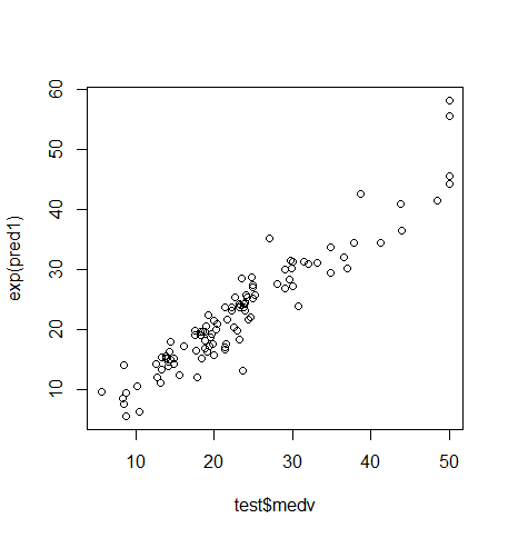
Till now we were checking training-error but the real goal of the model is to reduce the testing error. As we already split the sample dataset into training and testing dataset, we will use test dataset to evaluate the model that we have arrived upon. We will make a prediction based on ‘Model 4’ and will evaluate the model. As the last step, we will predict the ‘test’ observation and will see the comparison between predicted response and actual response value. RMSE explains on an average how much of the predicted value will be from the actual value. Based on RMSE = 3.278, we can conclude that on an average predicted value will be off by 3.278 from the actual value.pred1 <- predict(model4, newdata = test)
rmse <- sqrt(sum((exp(pred1) - test$medv)^2)/length(test$medv))
c(RMSE = rmse, R2=summary(model4)$r.squared)
c(RMSE = rmse, R2=summary(model4)$r.squared)
RMSE R2
3.2782608 0.7946003
par(mfrow=c(1,1))
plot(test$medv, exp(pred1))

Conclusion
The example shows how to approach linear regression modeling. The model that is created still has scope for improvement as we can apply techniques like Outlier detection, Correlation detection to further improve the accuracy of more accurate prediction. One can as well use an advanced technique like Random Forest and Boosting technique to check whether the accuracy can be further improved for the model. A piece of warning is that we should refrain from overfitting the model for training data as the test accuracy of the model will reduce for test data in case of overfitting.Reference
- 1. Statistics for Business By Robert Stine, Dean Foster
2. An Introduction to Statistical Learning, with Application in R. By James, G., Witten, D., Hastie, T., Tibshirani, R.


0 comments:
Post a Comment